The Johnson-Neyman technique and an R script to apply it

Versión en español aquí

UPDATE: the script presented in this post is now part of a more complete and easy to use R package: JNplots !! Go check the post about it, and the paper !

––––––––––––––––––––––––––––––––––––––––––––––––––––––––––––––––––––––––––––––

When starting to write this post I wanted to give a small introduction to the analysis of covariance (ANCOVA), because this post is in part based on that analysis. However, it might be better for you to review it by yourself if you need to.

As for any other statistical method ANCOVA assumes that certain conditions are met by the data. Depending on the question that you want to answer with ANCOVA, some of these assumptions might or might not be necessary to be met by the data (look here for a review about this subject)

However, there is an assumption that must be met if one wants to determine differences between groups. This is the assumption of homogeneity of the regression slopes.

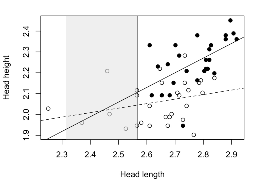
Let’s imagine that we want to compare the height of the head between males and females of a species of lizard (in lizards, taller heads are generally related to the consumption of larger prey and also to a better performance fighting against other individuals). Knowing that the head height in these animals covaries in respect to the head length we perform an ANCOVA. In the following figure we see the regression lines of males (black dots) and females (white dots) that represent the relationship between head height and length, and clearly we can notice that the assumption of homogeneity of the regression slopes is not met. It is enough to see how the regression lines are quite different in their “inclination”.

Head height vs head length in a lizard species. Black and white dots represent males and females respectively. Continuous and discontinuous lines represent the regression lines for males and females respectively.

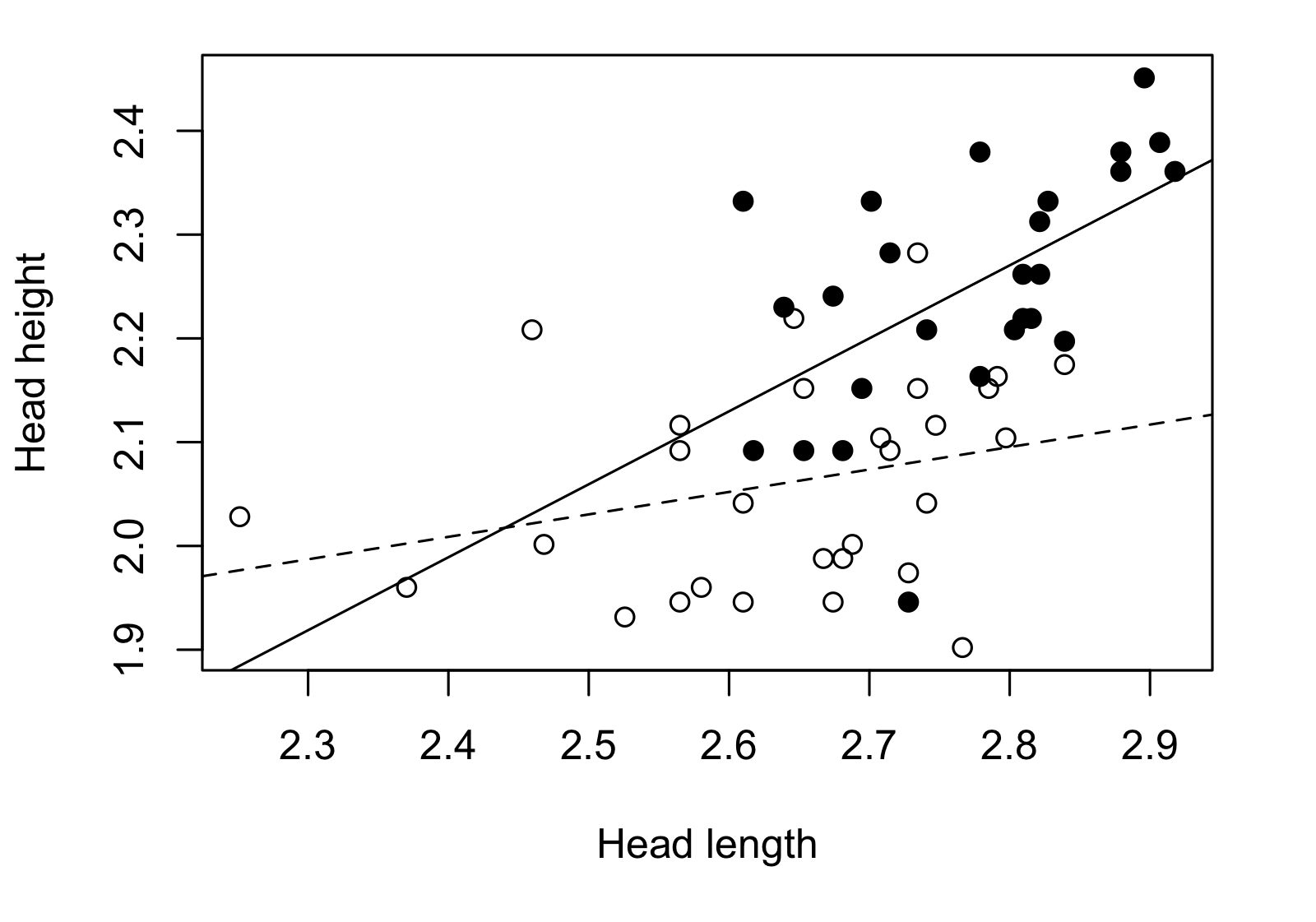
This will be confirmed if we perform the ANCOVA because the interaction between covariate (head length) and independent variable (sex) will be significant, indicating that the slopes are significantly different. Once the ANCOVA confirms this we can not compare between sexes using this method. What to do in this case?

I had this problem and, surprisingly, the solution was not that easy to find. I was a bit frustrated because, as you can see in the previous figure, is quite obvious that for a given head length males show higher heads than females, but I was not able to prove it statistically. My search became something similar to what you would expect from a detective novel, and from paper to paper I finally found a somewhat obscure method but that was supposed to solve my exact problem. This was the Johnson-Neyman technique.

Things of this method that surprised me:

– How hard was to find it.

– The precision with which it solved my problem.

– Its age! The original paper was published in 1936.

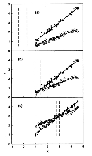
The JN technique is useful to solve cases like mine in which the regression slopes of the groups that I want to compare are different. This method generates a “non-significance zone”, that is basically an interval in the covariate within which there are no significant differences between groups. It is outside this interval where the groups are significantly different in respect to the dependent variable. The next figure might be good to explain what the method is about.

In the three cases of this figure we see how the regression lines representing the relationship Y~X of two groups (black and white dots) show different slopes when compared between them. Because of this condition we can not compare the values of both groups with an ANCOVA. The Johnson-Neyman technique generates “non-significance zones” (intervals between dashed lines) in which the difference between groups is not significant. At the same time, it allows us to identify the zones in which these differences are significant. Extracted from White, 2003.

I didn’t read the original paper, but a more recent paper that more directly explained the method (White, 2003). After finding the method I needed, the next step was to find a software or R package/function that allowed me to apply it. The rarity of the method in the literature was also reflected in its implementation in statistical packages. I could only find some “drafts” of R scripts and even some SPSS codes that were not working for me.

So I decided to take a look at the mathematical basis of the method. Luckily, White’s paper showed the equations on which the JN technique was based. Even though they were somewhat tedious I decided to write an R script to be able to apply the method directly. I will leave the script at the end just in case it is useful for anyone.

Applying the method through my script I obtained the following result for our example in lizards:

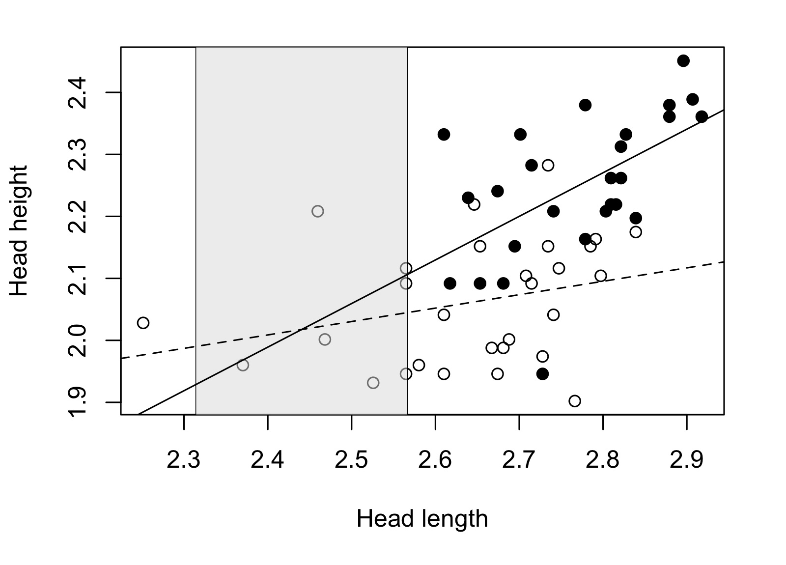
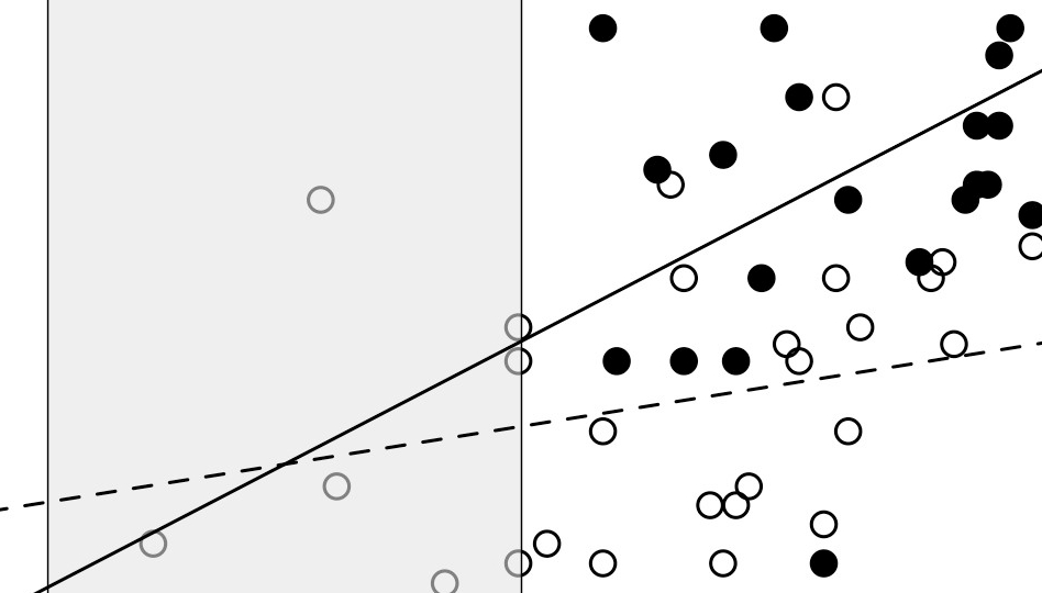
The non-significance zone is located in a head length interval for which there are almost no individuals to compare, actually there are no adult males in that zone. Most males and females are located out of the non-significance zone, where we can confidently affirm that the differences between males and females are significant. In consequence, we can conclude that adult males show higher heads than females for a given head length.

R script

Before starting, you need at least a dataset where rows are the cases and columns show the values of the dependent variable (in my example this was the head height), independent variable (e.g. sex) and covariate (e.g. head length).

The first step is then is to define your data table, which we will call “data”:

setwd("YourWorkingDirectory")
data <- read.table("YourData.txt",header=T, na.strings = c("x", "NA"))

I usually have my data in .txt format but the script can be modified to import excel (or you could convert your excel file to .txt)
The next step is to define your two* groups:

group1 <- data[ which(data$groups=="0"), ]
group2 <- data[ which(data$groups=="1"), ]

In this case I’m assuming that the column “groups” codifies both groups as “0” and “1”. This can vary in your own data.

So we define our groups as group1 and group2

*This script works for the case in which you want to compare 2 groups. I think the JN technique can be extended to consider more groups at the same time, but I did not look for more about how to do that.

In the next lines:

n1 <- 55
n2 <- 33

is necessary to change the number of cases there are for each group. In this case n1 corresponds to the number of cases of group1 and n2 corresponds to group2.

Finally:

X1 <- group1$hl
X2 <- group2$hl
Y1 <- group1$hh
Y2 <- group2$hh

you have to change the last part of each of these lines, both “hl” and “hh”. For me these letters meant head length or head height. This must be modified depending on how your dependent variable and the covariate are defined in your dataset.

After that you only need to run the rest of the code:

reg1 <- lm(log(Y1)~log(X1))
reg2 <- lm(log(Y2)~log(X2))
coef1 <- reg1$coefficients
coef2 <- reg2$coefficients
Fcvalue <- qf(.95, df1=1, df2=n1+n2-4)
xmean1 <- mean(log(X1))
xmean2 <- mean(log(X2))
xmeansq1 <- mean((log(X1))^2)
xmeansq2 <- mean((log(X2))^2)
sumx1 <- 0
sumx2 <- 0
sumy1 <- 0
sumy2 <- 0
sumxy1 <- 0
sumxy2 <- 0

xcoord_group1 <- log(X1) # X1
ycoord_group1 <- log(Y1) # Y1

xcoord_group2 <- log(X2) # X2
ycoord_group2 <- log(Y2) # Y2

zx1 <- ((sum(xcoord_group1))^2)/n1
zx2 <- ((sum(xcoord_group2))^2)/n2
zy1 <- ((sum(ycoord_group1))^2)/n1
zy2 <- ((sum(ycoord_group2))^2)/n2
zxy1 <- ((sum(xcoord_group1))*(sum(ycoord_group1)))/n1
zxy2 <- ((sum(xcoord_group2))*(sum(ycoord_group2)))/n2

######## sumx1 ########
c <- 0
while (c<n1) {
sumx1 <- sumx1 + (((xcoord_group1[c+1])^2) - zx1)
c <- c+1
}
sumx1

######## sumx2 ########
c <- 0
while (c<n2) {
sumx2 <- sumx2 + (((xcoord_group2[c+1])^2) - zx2)
c <- c+1
}
sumx2

######## sumy1 ########
c <- 0
while (c<n1) {
sumy1 <- sumy1 + (((ycoord_group1[c+1])^2) - zy1)
c <- c+1
}
sumy1

######## sumy2 ########
c <- 0
while (c<n2) {
sumy2 <- sumy2 + (((ycoord_group2[c+1])^2) - zy2)
c <- c+1
}
sumy2

######## sumxy1 ########
c <- 0
while (c<n1) {
sumxy1 <- sumxy1 + (((xcoord_group1[c+1])*(ycoord_group1[c+1]))-zxy1)
c <- c+1
}
sumxy1

######## sumxy2 ########
c <- 0
while (c<n2) {
sumxy2 <- sumxy2 + (((xcoord_group2[c+1])*(ycoord_group2[c+1]))-zxy2)
c <- c+1
}
sumxy2

########################
########################
########################
######## SSres ########

SSres <- (sumy1-(((sumxy1)^2)/sumx1))+(sumy2-(((sumxy2)^2)/sumx2))
SSres

########################
########################
########################
######## ABC ########
a1 <- coef1[1]
a2 <- coef2[1]
b1 <- coef1[2]
b2 <- coef2[2]
A <- (-Fcvalue/(n1+n2-4))*(SSres)*((1/sumx1)+(1/sumx2))+((b1-b2)^2)
B <- (Fcvalue/(n1+n2-4))*(SSres)*((xmean1/sumx1)+(xmean2/sumx2))+((a1-a2)*(b1-b2))
C <- (-Fcvalue/(n1+n2-4))*(SSres)*(((n1+n2)/(n1*n2))+(xmeansq1/sumx1)+(xmeansq2/sumx2))+((a1-a2)^2)

########################

xlower <- (-B-sqrt((B^2)-A*C))/A
xupper <- (-B+sqrt((B^2)-A*C))/A

xlower
xupper

xlower and xupper will indicate the inferior and superior limits of the non-significance zone respectively.

Plot

To generate this figure:

I used this code:

plot(log(data$hl),log(data$hh), ylab="Head height", xlab="Head length")
polygon(c(xlower,xlower,xupper,xupper),c(0,3.2,3.2,0),
col=rgb(224, 224, 224,maxColorValue=255,alpha=130), border=NA)
abline(v=xlower,lty=1, lwd=0.5)
abline(v=xupper,lty=1, lwd=0.5)
dat <- data[ which(data$group=="1"), ]
points(log(dat$hl),log(dat$hh), pch=16 ,col="black")
newdata <- data[ which(data$group=="1" ), ]
abline(lm(log(newdata$hh) ~ log(newdata$hl)))
newdata <- data[ which(data$group=="0" ), ]
abline(lm(log(newdata$hh) ~ log(newdata$hl)), lty=2)

References:

– Johnson, P. O., & Neyman, J. (1936). Tests of certain linear hypotheses and their application to some educational problems. Statistical research memoirs.

– White, C. R. (2003). Allometric analysis beyond heterogeneous regression slopes: use of the Johnson-Neyman technique in comparative biology. Physiological and Biochemical Zoology, 76(1), 135-140.

---

La técnica de Johnson-Neyman y un script de R para aplicarla

ACTUALIZACIÓN: el script presentado en este post es ahora parte de un paquete de R más completo y fácil de usar: JNplots !! Ve de qué se trata en este post, y lee el paper !

––––––––––––––––––––––––––––––––––––––––––––––––––––––––––––––––––––––––––––––

Al empezar a escribir este post quise dar una pequeña introducción al análisis de covarianza (ANCOVA), ya que el post se basa bastante en este análisis. Pero tal vez sea mejor que lo revises por tu cuenta si es que lo necesitas.

Como para cualquier método estadístico ANCOVA asume que ciertos supuestos son cumplidos por los datos. Dependiendo de la pregunta que se quiera resolver con el ANCOVA, algunos de estos supuestos podrían o no ser necesarios de cumplir (entra aquí para una revisión sobre el tema).

Sin embargo, hay un supuesto que sí debe ser cumplido si es que se quiere llegar a determinar diferencias entre grupos. Este es el supuesto de homogeneidad de las pendientes de regresión.

Imaginemos que queremos comparar el alto de cabeza entre machos y hembras de una especie de lagartija (en lagartijas, cabezas más altas generalmente están relacionadas al consumo de presas más grandes y también a un mejor desempeño en peleas con otros individuos). Sabiendo que el alto de la cabeza en estos animales covaría respecto al largo de la cabeza hacemos un ANCOVA. En la siguiente figura vemos las líneas de regresión para machos (puntos negros) y hembras (puntos blancos) que representan la relación entre alto de cabeza y largo de cabeza, y claramente podemos notar que el supuesto de homogeneidad de las pendientes de regresión no se cumple. Basta con ver cómo las líneas de regresión son bastante diferentes en su “inclinación”.

Alto de cabeza (head height) vs largo de cabeza (head length) en una especie de lagartija. Puntos negros y blancos representan machos y hembras respectivamente. Líneas continuas y discontinuas representan las lineas de regresión para machos y hembras respectivamente.

Esto será confirmado si hacemos el ANCOVA ya que la interacción entre covariante (largo de cabeza) y variable independiente (sexo) nos resultará significativa, indicando que las pendientes son significativamente diferentes. Una vez el ANCOVA confirma esto ya no podemos comparar entre sexos utilizando dicho método. ¿Qué se hace en este caso?

Yo me encontré con este problema y para mi sorpresa no me fue fácil encontrar una solución. Estaba algo frustrado ya que, como pueden ver en la figura, es bastante obvio que para un determinado largo de cabeza los machos muestran altos de cabeza mayores a los de las hembras, pero no podía demostrarlo estadísticamente. Mi búsqueda se convirtió en algo casi policial, y de paper en paper me encontré con una técnica bastante oscura pero que solucionaba el preciso problema con el que estaba lidiando. Esta es la técnica de Johnson-Neyman.

Cosas que me sorprendieron del método:

– Lo difícil que fue encontrarlo

– La precisión con la cual abordaba mi problema

– Su edad! El paper original fue publicado en 1936.

La técnica de JN se encarga de resolver casos como el mío, en los que las pendientes de las regresiones de los grupos que quiero comparar son distintas. Este método genera una “zona de no-significancia”, que es básicamente un intervalo en la covariante dentro del cual no hay diferencias entre grupos. Es en las zonas fuera de este intervalo donde los grupos muestran diferencias respecto a la variable dependiente. La siguiente figura explica mejor de qué se trata el método.

En los tres casos de esta figura vemos cómo las líneas de regresión representando la relación Y~X de dos grupos (puntos negros y blancos) muestran pendientes diferentes entre sí. Debido a esto no podemos comparar los valores de ambos grupos con un ANCOVA. La técnica de Johnson-Neyman genera “áreas de no-significancia” (intervalo representado por líneas discontinuas), en las cuales las diferencias entre grupos no son significativas. A su vez, nos permite identificar las zonas donde las diferencias sí lo son. Extraído de White, 2003.

No leí el paper original, sino un paper más moderno que explicaba el método de manera más directa (White, 2003). Luego de encontrar el método que necesitaba el siguiente paso era encontrar un software o paquete de R que me permitiera aplicarlo. La rareza del método en la literatura también se reflejaba en su implementación en paquetes estadísticos, solo pude encontrar algunos “bosquejos” de códigos de R e incluso SPSS que no me funcionaban.

Ante esto decidí mirar un poco la base matemática del método. Para mi suerte el paper de White mostraba las ecuaciones en las que el método de JN estaba basado. A pesar de que eran algo tediosas decidí escribir un script de R para poder aplicar el método de manera más directa. Dejaré el script al final por si algún día le sirve a alguien.

Aplicando el método a través de mi script obtuve el siguiente resultado para nuestro ejemplo en lagartijas:

La zona de no-significancia se ubica en un intervalo de largo de cabeza para el cual casi no hay individuos para comparar, de hecho no hay machos adultos en esa zona. La gran mayoría de hembras y machos se ubican fuera de la zona de no-significancia, donde podemos confirmar con tranquilidad que las diferencias entre machos y hembras son significativas. En consecuencia podemos concluir que machos adultos muestran altos de cabeza mayores que las hembras para un largo de cabeza determinado.

Script de R

 Para empezar necesitas al menos una base de datos donde las filas sean tus casos y las columnas muestren los valores de tu variable dependiente (en mi ejemplo esta era el alto de cabeza), variable independiente (e.g. sexo) y covariante (e.g. largo de cabeza).

El primer paso entonces es para definir tu tabla de datos, al que llamaremos “data”:

setwd("YourWorkingDirectory")
data <- read.table("YourData.txt",header=T, na.strings = c("x", "NA"))

Suelo tener mis datos en formato .txt pero el script se podría modificar para importar excel (o podrías convertir tu excel a .txt).

El siguiente paso es definir tus dos* grupos:

group1 <- data[ which(data$groups=="0"), ]
group2 <- data[ which(data$groups=="1"), ]

En este caso, estoy asumiendo que la columna “groups” codifica ambos grupos como “0” y “1”. Esto puede variar en tus propios datos.

Entonces, definimos nuestros dos grupos como group1 y group2.

*Este script aborda el caso en que quieras comparar dos grupos. Me parece que el método de JN se puede ampliar para considerar más grupos al mismo tiempo, pero no averigüé más acerca de cómo podría hacerse.
En la siguiente línea:

n1 <- 55
n2 <- 33

es necesario cambiar el número de casos que hay en cada grupo. En este caso n1 corresponde al número de casos de group1 y n2 corresponde a group2.

Finalmente:

X1 <- group1$hl
X2 <- group2$hl
Y1 <- group1$hh
Y2 <- group2$hh

tienes que cambiar la última parte de cada una de estas líneas, ya sea “hl” o “hh”. Para mí estas letras significaban “head length” (largo de cabeza) o “head height” (alto de cabeza). Esto debe ser modificado dependiendo de cómo tus variables dependiente y la covariante estén definidas en tu base de datos.

Luego de esto solo queda correr el resto del código:

reg1 <- lm(log(Y1)~log(X1))
reg2 <- lm(log(Y2)~log(X2))
coef1 <- reg1$coefficients
coef2 <- reg2$coefficients
Fcvalue <- qf(.95, df1=1, df2=n1+n2-4)
xmean1 <- mean(log(X1))
xmean2 <- mean(log(X2))
xmeansq1 <- mean((log(X1))^2)
xmeansq2 <- mean((log(X2))^2)
sumx1 <- 0
sumx2 <- 0
sumy1 <- 0
sumy2 <- 0
sumxy1 <- 0
sumxy2 <- 0

xcoord_group1 <- log(X1) # X1
ycoord_group1 <- log(Y1) # Y1

xcoord_group2 <- log(X2) # X2
ycoord_group2 <- log(Y2) # Y2

zx1 <- ((sum(xcoord_group1))^2)/n1
zx2 <- ((sum(xcoord_group2))^2)/n2
zy1 <- ((sum(ycoord_group1))^2)/n1
zy2 <- ((sum(ycoord_group2))^2)/n2
zxy1 <- ((sum(xcoord_group1))*(sum(ycoord_group1)))/n1
zxy2 <- ((sum(xcoord_group2))*(sum(ycoord_group2)))/n2

######## sumx1 ########
c <- 0
while (c<n1) {
sumx1 <- sumx1 + (((xcoord_group1[c+1])^2) - zx1)
c <- c+1
}
sumx1

######## sumx2 ########
c <- 0
while (c<n2) {
sumx2 <- sumx2 + (((xcoord_group2[c+1])^2) - zx2)
c <- c+1
}
sumx2

######## sumy1 ########
c <- 0
while (c<n1) {
sumy1 <- sumy1 + (((ycoord_group1[c+1])^2) - zy1)
c <- c+1
}
sumy1

######## sumy2 ########
c <- 0
while (c<n2) {
sumy2 <- sumy2 + (((ycoord_group2[c+1])^2) - zy2)
c <- c+1
}
sumy2

######## sumxy1 ########
c <- 0
while (c<n1) {
sumxy1 <- sumxy1 + (((xcoord_group1[c+1])*(ycoord_group1[c+1]))-zxy1)
c <- c+1
}
sumxy1

######## sumxy2 ########
c <- 0
while (c<n2) {
sumxy2 <- sumxy2 + (((xcoord_group2[c+1])*(ycoord_group2[c+1]))-zxy2)
c <- c+1
}
sumxy2

########################
########################
########################
######## SSres ########

SSres <- (sumy1-(((sumxy1)^2)/sumx1))+(sumy2-(((sumxy2)^2)/sumx2))
SSres

########################
########################
########################
######## ABC ########
a1 <- coef1[1]
a2 <- coef2[1]
b1 <- coef1[2]
b2 <- coef2[2]
A <- (-Fcvalue/(n1+n2-4))*(SSres)*((1/sumx1)+(1/sumx2))+((b1-b2)^2)
B <- (Fcvalue/(n1+n2-4))*(SSres)*((xmean1/sumx1)+(xmean2/sumx2))+((a1-a2)*(b1-b2))
C <- (-Fcvalue/(n1+n2-4))*(SSres)*(((n1+n2)/(n1*n2))+(xmeansq1/sumx1)+(xmeansq2/sumx2))+((a1-a2)^2)

########################

xlower <- (-B-sqrt((B^2)-A*C))/A
xupper <- (-B+sqrt((B^2)-A*C))/A

xlower
xupper

xlower y xupper indicarán los límites inferior y superior respectivamente de la zona de no significancia.

Plot

Para generar esta figura:

Utilicé este código:

plot(log(data$hl),log(data$hh), ylab="Head height", xlab="Head length")
polygon(c(xlower,xlower,xupper,xupper),c(0,3.2,3.2,0),
col=rgb(224, 224, 224,maxColorValue=255,alpha=130), border=NA)
abline(v=xlower,lty=1, lwd=0.5)
abline(v=xupper,lty=1, lwd=0.5)
dat <- data[ which(data$group=="1"), ]
points(log(dat$hl),log(dat$hh), pch=16 ,col="black")
newdata <- data[ which(data$group=="1" ), ]
abline(lm(log(newdata$hh) ~ log(newdata$hl)))
newdata <- data[ which(data$group=="0" ), ]
abline(lm(log(newdata$hh) ~ log(newdata$hl)), lty=2)

Referencias:

– Johnson, P. O., & Neyman, J. (1936). Tests of certain linear hypotheses and their application to some educational problems. Statistical research memoirs.

– White, C. R. (2003). Allometric analysis beyond heterogeneous regression slopes: use of the Johnson-Neyman technique in comparative biology. Physiological and Biochemical Zoology, 76(1), 135-140.